I’m currently taking Differential Equations in school and during class Euler’s method was a brief topic of discussion. Euler’s method is really simple, but it works really well. As my teacher puts it, we “dumbass” our way to the right answer. There are better methods than it that have faster convergence, less error, or more efficiency, but during my journey of trying to learn about them, I’ve found that they’re explained with unnecessary complexity. In this post, I’m going to explore Euler’s method, as well as a more powerful extension of it. In another post, coming soon, I’ll try to intuitively explain the more complex improvements made on Euler’s method.
Euler’s Method 
Let’s quickly review how Euler’s method works. The idea is very simple, but we need a few things: a differential equation like \(\frac{dy}{dt} = f(x, y)\) , and some initial value \( y(x_0) = y_0 \) . Once we have these, we can apply our understanding of tangent lines and follow the curve.
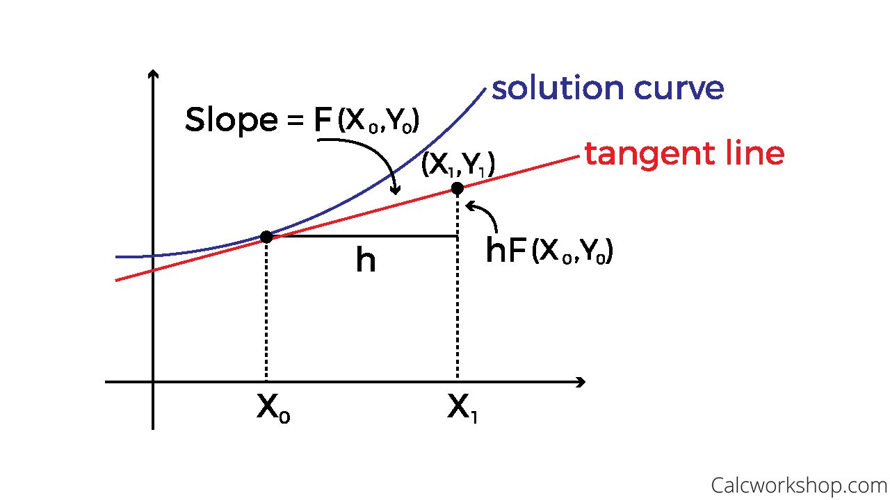
Since the slope of the tangent line is equivalent to the deriviative at that point, we can approximate \( y(x_0 + h) \) with the equation \( y_{1} = y_0 + h*f(x_0, y_0) \) . Then, we can keep iterating, generalizing to: \( y_{n + 1} = y_n + h*f(x_n, y_n) \) , while \( x \) increases by \( h \) at every step. We just keep following the tangent line and hope that we are close to the actual function, and, surprisingly enough, this works pretty well for most differential equations. This specific idea is called the explicit Euler method. We’ll take a look at what it means to be implicit, not explicit, in a moment.
Implementing Euler’s Method 
This is, after all, a programming blog, so it would be unfair to not implement Euler’s method in Python. We’ll take a higher-order numpy-compliant function as our input, as well as the initial condition and the step size, and then just iterate.
# endpoints is a tuple of (x_0, x_n), where x_n is our ending point
def euler_explicit(f_prime, y_0, endpoints, h):
    n = int((endpoints[-1] - endpoints[0])/h) # number of steps
    x = endpoints[0]
    y = y_0
    x_out, y_out = np.array([x]), np.array([y])
    for i in range(n):
        y_prime = f_prime(x, y)
        y += h * y_prime # y_n+1 = y_n + h * f
        x += h
        x_out = np.append(x_out, x)
        y_out = np.append(y_out, y)

    return x_out, y_out
That’s really clean! How does it do? Let’s take a look at a simple example:
def exp_prime(x, y):
  return y

def exp_sol(x):
  return np.exp(x)

x_euler, y_euler = euler_explicit(exp_prime, 1, (0, 1), 0.1)
x = np.arange(0, 1, 0.01)
y = exp_sol(x)
We get:
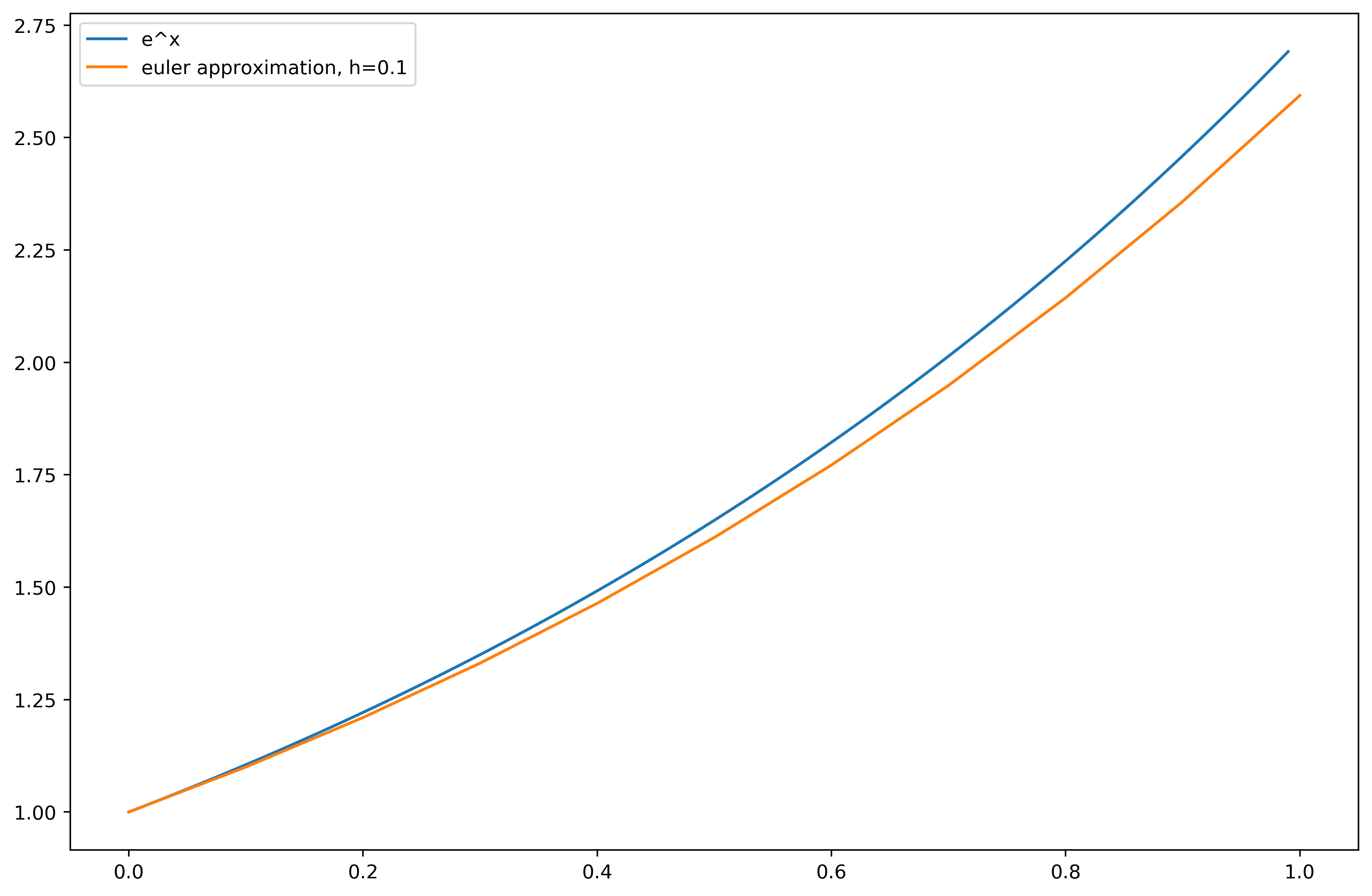
We can do better than this
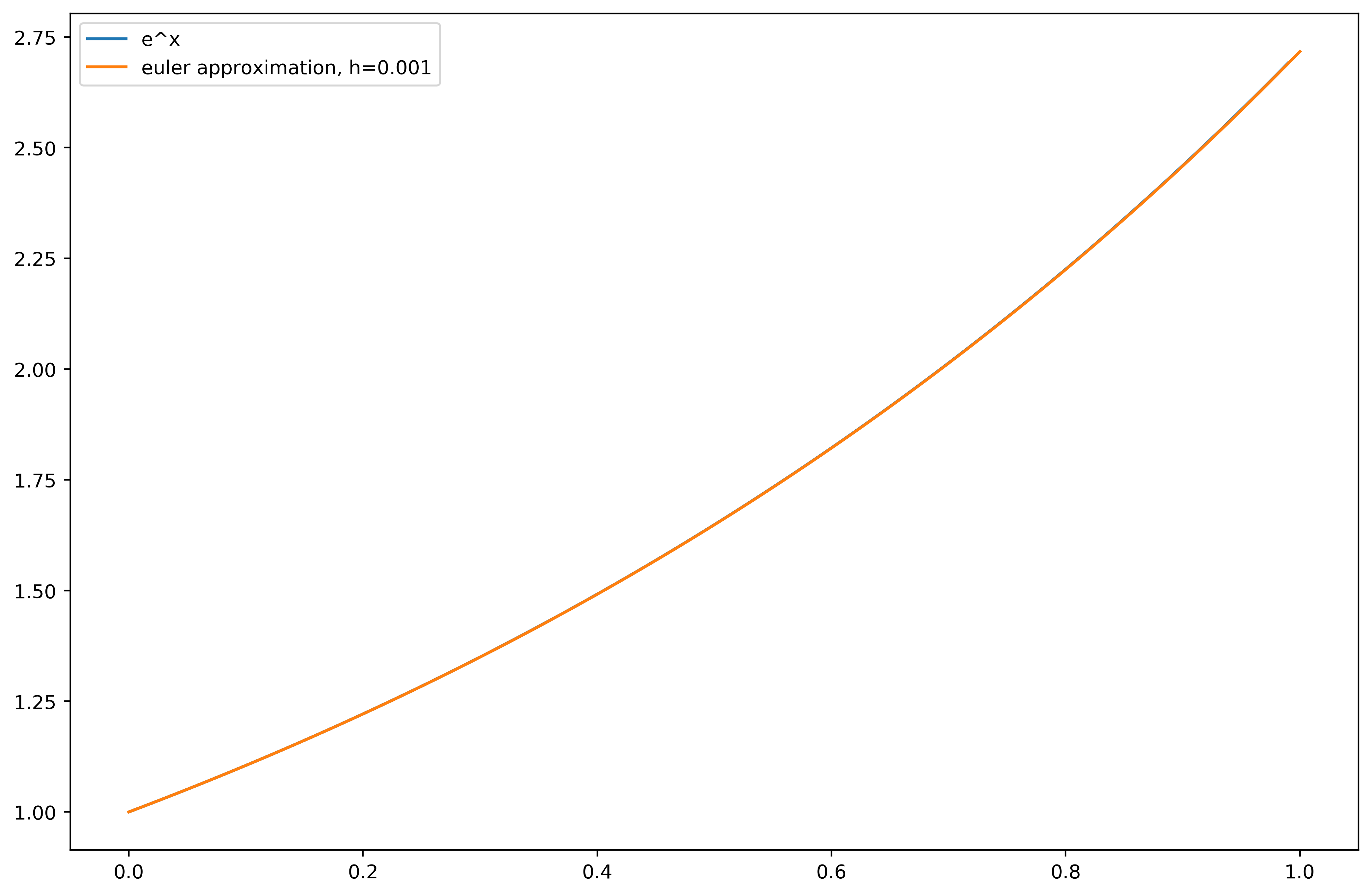
Not great, if we graph the error we’ll see that it grows at a non-linear rate, but I’m being mean to Euler. A step size of 0.1 is really big, and modern computers can handle a lot smaller. With a step of 0.001, we get:
Nice. There are many cases though, where Euler’s method is inaccurate even for small steps, or it is “unstable” and oscillates around the right answer. For example,
\( y' = -8y \)
:
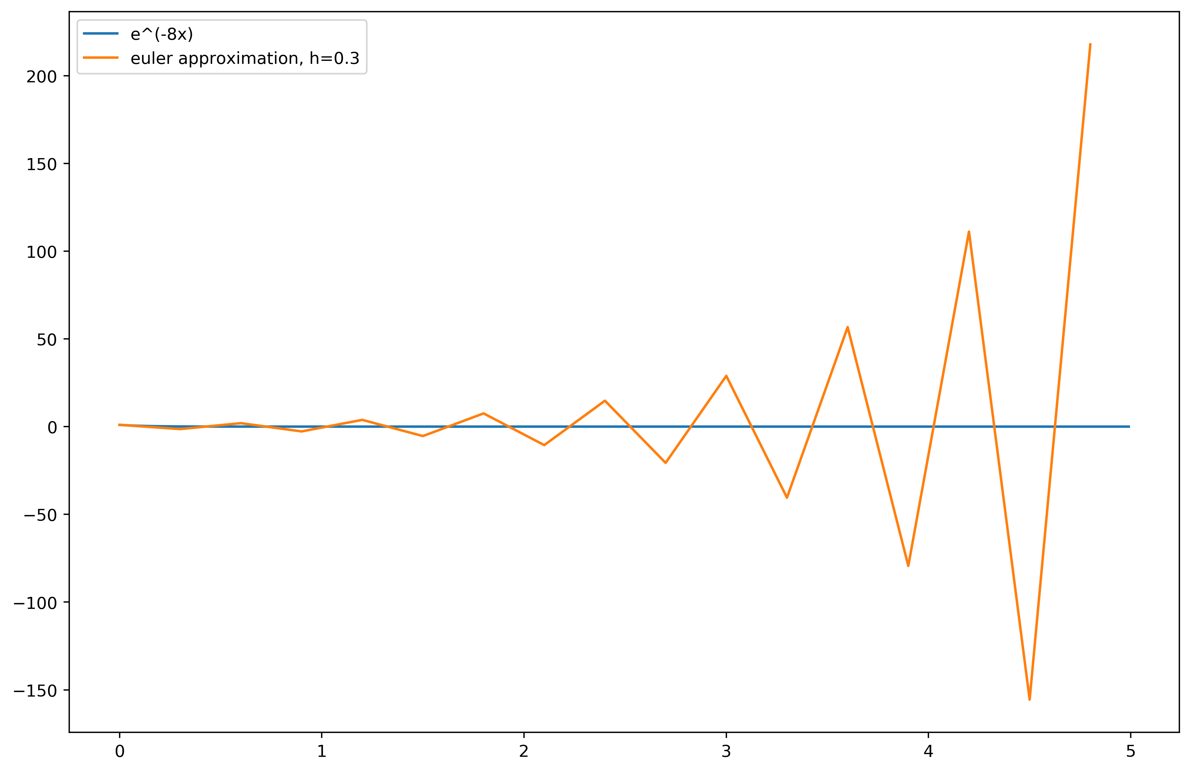
Making sure that you’re approximation function is stable and is coming close to the right answer is much more math than what I’m hoping to get into (or that I even understand, yet), but we can look at some methods of approximation that are less likely to be unstable or produce faster, better results.
Implicit Euler? 
Euler’s method looks forward using the power of tangent lines and takes a guess. Euler’s implicit method, also called the backward Euler method, looks back, as the name implies. We’ve been given the same information, but this time, we’re going to use the tangent line at a future point and look backward. So, our approximation is instead: \( y_{n+1} = y_n + h f(x_{n+1}, y_{n+1}) \) . If you’ve been paying attention, you are angry at me. We don’t know what \( y_{n+1} \) is, but it shows up on both sides of the equation. That sucks, and it is why this is called the implicit Euler: there is no explicit answer. We can however, do some math and find \( y_{n+1} \) in terms of our original function.
With our implicit equation, we know that \( y(x + h) = y(x) + hf(y(x + h)) \) , but for our specific example, \( f = -8y \) , we can just plug this in!
$$ y(x + h) = y(x) -8hy(x + h) $$ $$ = \frac{y(x)}{1 + 8h} $$
Now, if you can’t solve the equation that you’re given, you can use any root-finding algorithm (a lot of the books I’ve seen recommend Newton’s), to find a solution. This is much more intensive than the explicit method, as it either requires human intervention or a root-finding algorithm, so does it pay off?
Let’s implement implicit euler specifically for our given equation:
def euler_implicit_8y(f_prime, y_0, endpoints, h):
    n = int((endpoints[-1] - endpoints[0])/h)
    x = endpoints[0]
    y = y_0
    x_out, y_out = np.array([x]), np.array([y])
    for i in range(n):
        y_prime = f_prime(x, y)/(1 + h * 8)
        y += h * y_prime
        x += h
        x_out = np.append(x_out, x)
        y_out = np.append(y_out, y)

    return x_out, y_out
So, what happens with
\( h = 0.3? \)
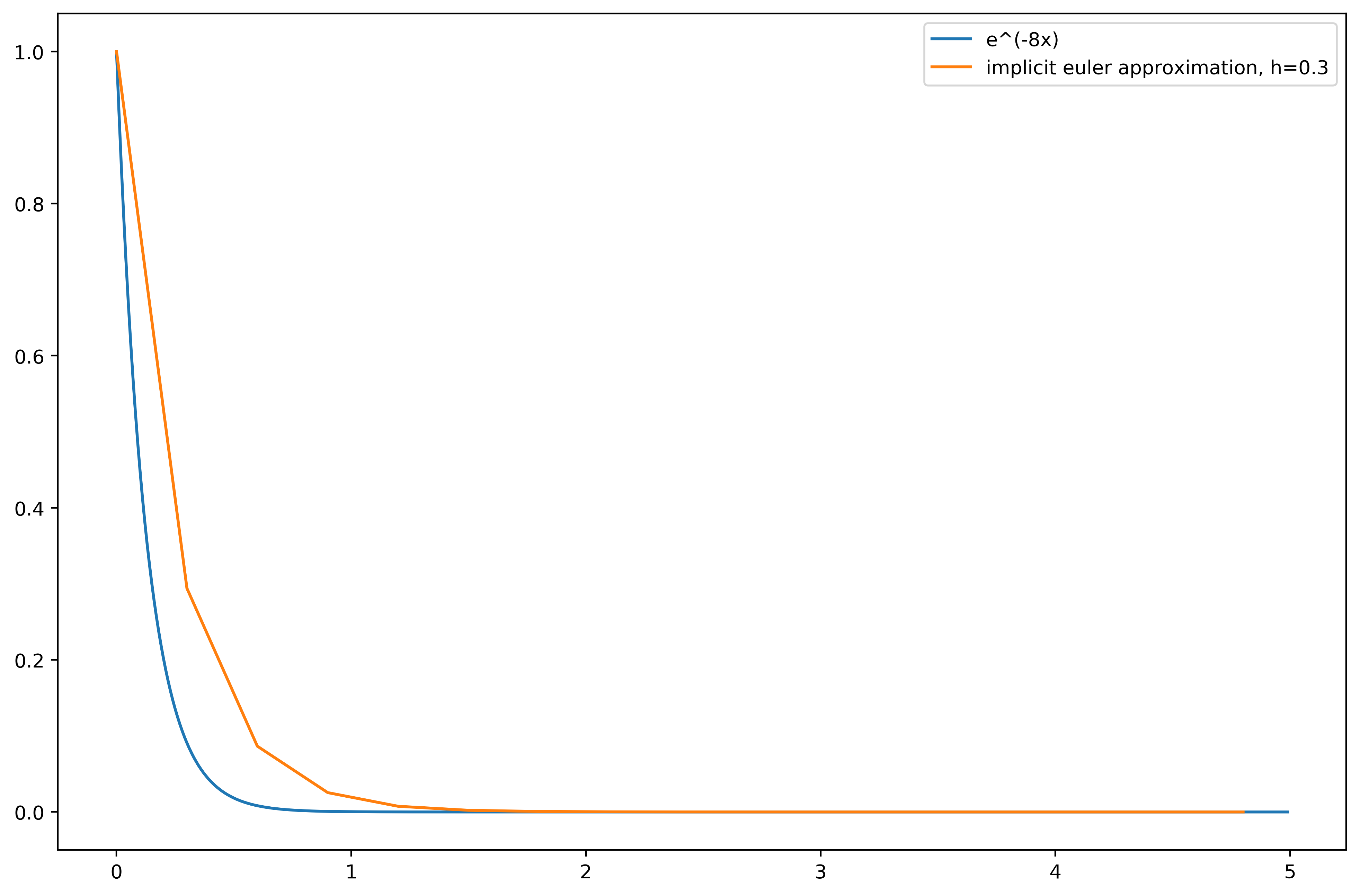
Nice! We can even increase our h to a much larger number, and still get a result that eventually converges. For a little bit of human analysis (that could be removed by using a root-finding algorithm), we got a method that will always converge. It is possible to determine whether, and under what step sizes, the implicit Euler will converge, but this is something that I don’t have a great grasp on yet. As you can see, using an implicit method is more expensive computationally, but worth it if convergence is an issue.
Keep an eye out, as, during my deep dive into numerical analysis, I’ve been bothered by the overly complex explanations for rather simple ideas, like Heun’s method and Runge-Kutta, so I’ll be going over those soon.