Extending Euler’s method

Last time, I discussed two of Euler’s methods for numerical approximation, explicit and implicit Euler. In this blog post, we’re going to extend the idea of Euler’s method, and then generalize our extension into something called Runge-Kutta. I apologize for the delay between blog posts, I’ve been working on college apps, but I hope to get a bit more active now, especially with the Advent of Code going on.

Extended Euler (or Heun’s Method) ¶

When we worked with explicit Euler, we stepped forward by \( h \) , but we found the slope only at our given \( (x, y) \) . What if we instead found the slope at \( (x, y) \) and the slope at \( (x+h, y_1) \) and then averaged those? This method is pretty simple, just as simple as the normal Euler method, and it is much more accurate.

Here’s a quick visualization:

The idea behind this extension is super intuitive, and the formal math isn’t complex either.

$$ \tilde{y}_{i+1} = y_i + h \cdot f’(x_i,y_i) $$

$$ m = \frac{1}{2} \cdot [f’(x_i, y_i) + f’(x_{i+1}, \tilde{y_{i+1}})] $$

$$ y_{i+1} = y_i + m \cdot h$$

We can implement this in Python, as we’ve been doing, as so:

def heun(f_prime, y_0, endpoints, h):
    n = int((endpoints[-1] - endpoints[0])/h)
    x = endpoints[0]
    y = y_0
    x_out, y_out = np.array([x]), np.array([y])
    for i in range(n):
        y_intermediate = y + h*f_prime(x, y)

        y += (h/2) * (f_prime(x, y) + f_prime(x+h, y_intermediate))


        x += h
        x_out = np.append(x_out, x)
        y_out = np.append(y_out, y)

    return x_out, y_out

Extending Extended Euler? (Runge-Kutta) ¶

What if we kept going? Instead of taking 2 slopes, let’s take 3, or 4, or even 1000, and average them. Maybe we can do a weighted average? This is the fundamental idea behind the Runge-Kutta method of approximators. The most common Runge-Kutta approximation is with 4 points, often called RK4. Let’s look at it:

This is a lot more complex than what we were looking at before, but the ideas are the same. We are computing the slope at the initial point that we start at, and then we are using that slope to calculate more points, slowly oscillating around a final answer.

RK4 has some really useful applications. It is very accurate, so it’s often used in approximating systems of differential equations. The Van der Pol oscillator is a very common example that is used to demonstrate its power. Let’s do something a little more relevant, such as modeling the spread of a disease.

We have to adapt our code so that we use an array of starting points and give the differential equation a vector of points. This is really easy to do with numpy.

def rk4(f_prime, y_0, endpoints, h):
    n = int((endpoints[-1] - endpoints[0]) / h)

    x = endpoints[0]
    y = np.copy(y_0) # note that y_0 is now an np.array rather than an integer

    x_out, y_out = np.array([x]), np.array([y])

    for i in range(n):
        k1 = f_prime(x, y)

        yp2 = y + k1*(h/2)

        k2 = f_prime(x+h/2, yp2)

        yp3 = y + k2*(h/2)

        k3 =  f_prime(x+h/2, yp3)

        yp4 = y + k3*h

        k4 = f_prime(x+h, yp4)
        y += (h/6)*(k1 + 2*k2 + 2*k3 + k4)

        x = x + h
        x_out = np.append(x_out, x)

        y_out = np.vstack((y_out, y)) # note that we are using vstack here, so we have to transpose when outputting

    return x_out, y_out.T # transposing to make our output consistent

We can use RK4 with a SIR model to approximate the spread of a disease. We can create a function to represent the SIR model like so:

def SIR(infection_rate=0.684, recovery_rate=1/28, pop=2400):
    def SIR_diffeq(x, y):
        dy = np.zeros(len(y))
        dy[0] = -infection_rate * y[0]/(pop) * y[1]
        dy[1] = y[1]*(infection_rate*y[0]/(pop) - recovery_rate)
        dy[2] = recovery_rate * y[1]
        return dy
    return SIR_diffeq # first-class functions are awesome
standard_SIR = SIR()

The values given for constants were what I used for a class assignment where we had to approximate the spread of COVID in a school. I am not an epidemiologist, and I think most epidemiologists would scoff at using an SIR model to actually approximate the spread of a disease, so please don’t take these values seriously in any way.

Plotting our equation:

h = 0.01
x = np.array([0.0, 30.0])
yinit = np.array([2395.0, 5.0, 0.0])
x, y = rk4(standard_SIR, yinit, x, h)

We get:

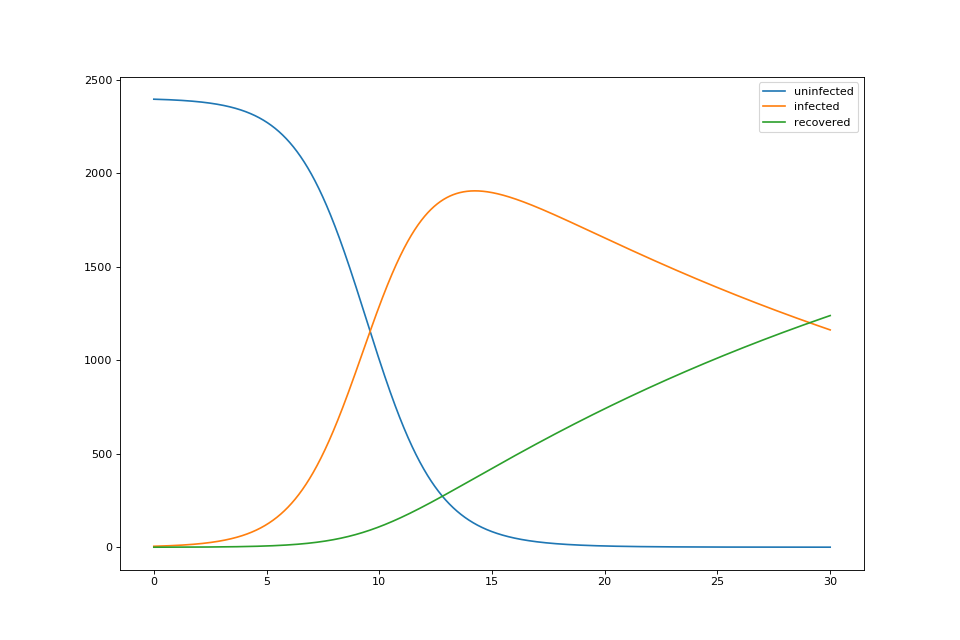
That’s super cool, and obviously, there are more domain-specific examples where the accuracy of RK4 becomes relevant. We could’ve done the same with explicit Euler and gotten just as good of an answer when it comes to the SIR model.

Generalizing Runge-Kutta ¶

The reason this is called RK4 is because we calculate 4 different slopes, but then there’s also the weights that we assign to each slope. We can generalize the RK methods by creating something called a Butcher tableau (named after J.C. Butcher). We write a tableau for RK4 as such:

The bottom row is our set of weights, and the left side is the coefficients of our step size. If you look back at RK4, you can see that we move up by 1/2 of the step size, until our final step, where we compute the value at our final point. As we move across the row from left to right, each column represents a specific \( k \) . If we wanted to define more complex approximators, we could factor in previous \( k \) s, but in RK4 we ignore all the slopes except the current.

We can also write Heun’s method:

or even Euler’s method:

Although we can create more complex tableaus and create approximators that keep simplifying the slope thousands of times, there’s a point that it stops being computationally worthwhile. I’m still exploring this math myself, so I can’t answer how you know to stop, but I do know that in practice, people rarely use approximators more complex than RK4.